List of the Top 10 Excel Formulas for Data

As a data analyst, I rely on Excel as one of the most powerful tools every day. It’s not just about organizing data; it’s about turning that data into something meaningful. One of the most powerful aspects of Excel is its formulas. These formulas are the backbone of transforming raw data into actionable insights.

In this article, I will walk you through the top 10 Excel formulas every data analyst must master. I’ll break them down with simple examples so you can apply them immediately. If you want to skip the data collection and cleaning, check out my list of the best dataset providers.

As a data analyst, mastering Excel formulas is crucial for turning raw data into actionable insights. These formulas streamline data analysis, helping you uncover patterns, perform calculations, and make informed decisions. Here are 10 essential Excel formulas that every data analyst should have in their toolkit.

1. SUM

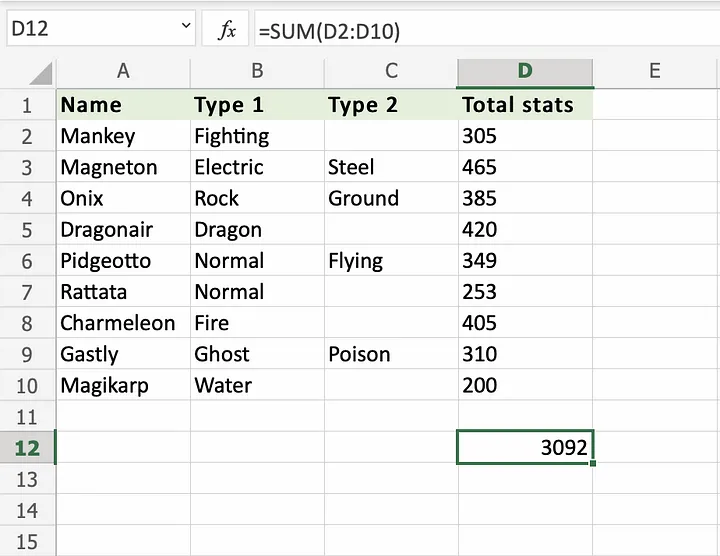
The SUM function is the most basic yet one of the most useful Excel functions. It allows you to add up numbers across a range of cells. For instance, if you’re analyzing sales data, you can quickly sum up total sales over a specific period.

Syntax: =SUM(number1, [number2], …)

Example: If you have sales data in cells A2 to A10, you can sum it using =SUM(A2:A10).

Use Case: Summing data is often the first step in data analysis, quickly assessing total values across datasets.

2. AVERAGE

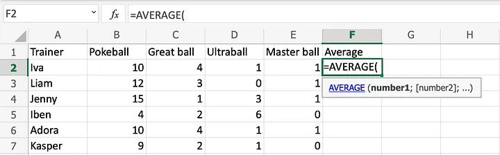
The AVERAGE function calculates the mean of a range of numbers. It’s useful when you want to determine the average value in a dataset, such as average sales per month or the average score of survey respondents.

Syntax: =AVERAGE(number1, [number2], …)

Example: To find the average score of students from cells B2 to B15, use =AVERAGE(B2:B15).

Use Case: AVERAGE is essential when analyzing data trends over time. It helps to smooth out short-term fluctuations and reveal underlying trends.

3. IF

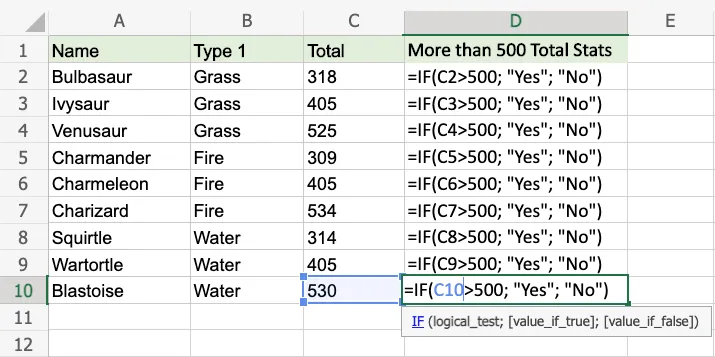
The IF function is a conditional formula that performs different actions based on whether a given condition is true or false. It’s compelling for categorizing data, such as marking sales as “high” or “low” based on a threshold.

Syntax: =IF(logical_test, value_if_true, value_if_false)

Example: To label sales in cell C2 as “High” if the value is greater than 1000 and “Low” otherwise, use =IF(C2>1000, “High”, “Low”).

Use Case: The IF function is invaluable for segmenting data into meaningful categories, enabling more targeted analysis.

4. VLOOKUP

VLOOKUP (Vertical Lookup) is one of the most frequently used Excel functions for finding data in a large table or database. It searches for a value in the first column of a table and returns a value in the same row from another column.

Syntax: =VLOOKUP(lookup_value, table_array, col_index_num, [range_lookup])

Example: To find the price of a product with ID 103 in a table located in A2

, use =VLOOKUP(103, A2:C10, 3, FALSE).

Use Case: VLOOKUP is perfect for combining data from different tables based on a common key, such as matching customer names with their respective purchases.

5. HLOOKUP

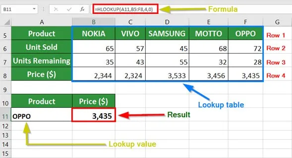
HLOOKUP (Horizontal Lookup) works similarly to VLOOKUP, but it searches for a value in the top row of a table and returns a value in the same column from another row.

Syntax: =HLOOKUP(lookup_value, table_array, row_index_num, [range_lookup])

Example: To find the sales figure for March in a row labeled with months, use =HLOOKUP(“March”, A1:H3, 3, FALSE).

Use Case: HLOOKUP is ideal when your data is organized horizontally, and you need to retrieve information from a specific column.

6. INDEX and MATCH

INDEX and MATCH are often used as an alternative to VLOOKUP and HLOOKUP. They are more flexible, allowing you to look up values in any column or row, not just the first one.

Syntax:

• INDEX(array, row_num, [column_num])
• MATCH(lookup_value, lookup_array, [match_type])

Example: To find the price of a product with ID 103 using INDEX and MATCH, use: =INDEX(C2:C10, MATCH(103, A2:A10, 0)).

Use Case: INDEX and MATCH are powerful for complex lookups where VLOOKUP falls short, especially when the lookup column isn’t the first in your data range.

7. COUNTIF

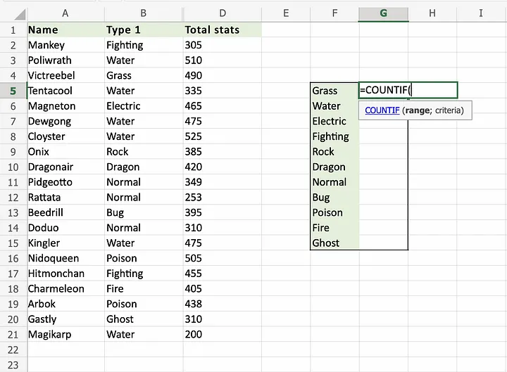
COUNTIF counts the number of cells within a range that meet a single condition. It’s useful for quickly tallying items that match specific criteria, such as counting the number of sales above a certain amount.

Syntax: =COUNTIF(range, criteria)

Example: To count how many cells in the range B2

have sales above 500, use =COUNTIF(B2:B10, “>500”).

Use Case: COUNTIF is great for quick data summaries, helping to identify how often a particular condition is met within your dataset.

8. SUMIF

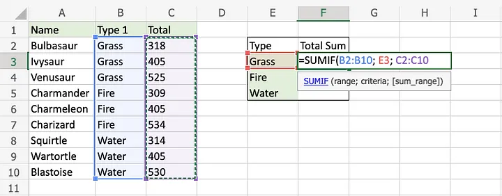
SUMIF combines the power of SUM and IF, allowing you to add values in a range that meets specific criteria. It’s excellent for financial analysis, like summing up expenses that exceed a certain amount.

Syntax: =SUMIF(range, criteria, [sum_range])

Example: To sum sales in column B where the value in column A is “Product A”, use =SUMIF(A2:A10, “Product A”, B2:B10).

Use Case: SUMIF is ideal for aggregating data based on specific conditions, enabling targeted analysis of particular segments.

9. CONCATENATE (or TEXTJOIN)

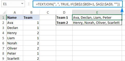
CONCATENATE (or its modern counterpart TEXTJOIN) allows you to combine text from multiple cells into one. This is useful for creating labels, full names, or combining data from different sources.

Syntax:

• =CONCATENATE(text1, [text2], …)
• =TEXTJOIN(delimiter, ignore_empty, text1, [text2], …)

Example: To combine the first name in A2 and the last name in B2, use =CONCATENATE(A2, “ “, B2) or =TEXTJOIN(“ “, TRUE, A2, B2).

Use Case: CONCATENATE is handy for preparing data for reports, especially when creating composite labels or merging text data from different sources.

10. PIVOT TABLES

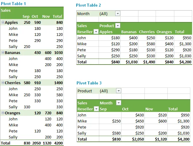
While not a formula in the traditional sense, Pivot Tables are an advanced Excel feature that allows you to summarize and analyze large datasets dynamically. They enable you to reorganize, filter, and summarize your data without altering the original dataset.

Example: You can use a Pivot Table to summarize sales data by region, product, or any other category.

Use Case: Pivot Tables are essential for data analysis. They allow you to explore relationships within your data, identify trends, and generate reports easily.

Conclusion

Mastering these top 10 Excel formulas has greatly improved my data analysis skills. Whether you’re just starting or looking to enhance your abilities, these functions are essential in any data analyst’s toolkit. These Excel formulas, from simple sums to advanced lookups and Pivot Tables, help me extract insights, identify patterns, and make informed decisions. Excel is a crucial tool for data analysis.

Understanding these formulas provides a strong foundation for more complex data manipulation and analysis tasks. As I continue to explore Excel’s features, I find that these functions not only save time but also open up new ways to explore and interpret data.